Introduction
The iraceplot package provides a set of functions to create plots to visualize the configuration data generated by the configuration process implemented in the irace package.
The configuration process performed by irace will show ar the end of the execution one or more configurations that are the best performing configurations found. This package provides a set of functions that allow to further assess the performance of these configurations and provides support to obtain insights about the details of the configuration process.
Installation
Install iraceplot from CRAN
install.packages("iraceplot")Install iraceplot from github
For installing iraceplot you need to install the devtools package:
install.packages("devtools")
devtools::install_github("auto-optimization/iraceplot/")
Executing irace
To use the methods provided by this package you must have an irace data object, this object is saved as an Rdata file (irace.Rdata by default) after each irace execution.
During the configuration procedure irace evaluates several candidate configurations (parameter settings) on different training insrances, creating an algorithm performance data set we call the training data set. This information is thus, the data that irace had access to when configuring the algorithm.
You can also enable the test evaluation option in irace, in which a set of elite configurations will be evaluated on a set of test instances after the execution of irace is finished. Nota that this option is not enabled by default and you must provide the test instances in order to enable it. The performance obtained in this evalaution is called the test data set. This evaluation helps assess the results of the configuration in a more “real” setup. For example, we can assess if the configuration process incurred in overtuning or if a type of instance was underrepresented in the training set. We note that irace allows to perform the test evaluations to the final elite configurations and to the elite configurations of each iterations. For information about the irace setup we refer you to the irace package user guide.
Note: Before executing irace, consider enabling testing
in irace.
Once irace is executed, you can load the irace log in the R console as previously shown.
Load irace log data
You can load the data from the log file as follows:
iraceResults <- irace::read_logfile("~/path/to/irace.Rdata")For more details about the contents of the log file, please go to the user guide of the irace package.
However, most functions directly accept a filename and do not require you to load the data yourself. We only mention here for completeness.
Visualizing irace configuration data
In the following, we provide an example how the functions implemented in this package can be used to visualize the information generated by irace.
Configurations
Once irace is executed, the first thing you might want to do is to
visualize how the best configurations look like. You can do this with
the parallel_coord method:
parallel_coord(iraceResults)The plot shows by default the final elite configurations (last
iteration), each line in the plot represents one configuration. The plot
produced by parallel_coord can help you to both the
distribution of the parameter values of a set of configurations and the
common associations between these values. By default, the plot colors
the lines using the number of instances evaluated by the configuration.
You can use the color_by_instances argument to choose
between coloring the lines by the number of instances executed or the
last iteration the configurationwas executed on.
To visualize the configurations considered as elites in each
iteration use the iterations option. You can select one or
more iterations. For example, to select all iterations executed by
irace:
parallel_coord(iraceResults, iterations=1:iraceResults$state$nbIterations,
               color_by_instances = FALSE)
You can also visualize all configurations sampled in one or more
iterations disabling the only_elite option. For example, to
visualize configurations sampled in iterations 1 to 9:
parallel_coord(iraceResults, iterations=1:9, only_elite=FALSE)If you are looking for something more flexible and you would like to
provide your own set of configurations, you can use the
plot_configurations() function. This function generates a
parallel coordinates plot (similar to the ones generated by
parallel_coord()) when provided with an arbitrary set of
configurations and a parameter space object. The configurations must be
provided in the format in which irace handles configurations: a
dataframe with parameter in each column. For information about these
formats, please chech the irace package user
guide. As an example, this lines display all elite
configurations:
all_elite <- iraceResults$allConfigurations[unlist(iraceResults$allElites),]
parameters <- iraceResults$scenario$parameters
plot_configurations(all_elite, parameters)
The parallel_cat function displays all configurations
sampled in a set of iterations. The plot groups parameter values in
intervals and thus, it can be useful to visualize more tendencies of
association between parameters values. As in the previous functions you
can use the iterations argument to select the iterations
from which configurations should be selected. For example, to visualize
configurations sampled on iterations 3, 4 and 5:
parallel_cat(irace_results = iraceResults, iterations = c(3,4,5) )## Warning in set(tabla, i = which(not_na), j = pname, value = bins): Coercing
## 'character' RHS to 'double' to match the type of column 5 named 'alpha'.## Warning in set(tabla, i = which(not_na), j = pname, value = bins): NAs
## introduced by coercion## Warning in set(tabla, i = which(is.na(tabla[[pname]])), j = pname, value =
## "NA"): Coercing 'character' RHS to 'double' to match the type of column 5 named
## 'alpha'.## Warning in set(tabla, i = which(is.na(tabla[[pname]])), j = pname, value =
## "NA"): NAs introduced by coercion## Warning in set(tabla, i = which(not_na), j = pname, value = bins): Coercing
## 'character' RHS to 'double' to match the type of column 6 named 'beta'.## Warning in set(tabla, i = which(not_na), j = pname, value = bins): NAs
## introduced by coercion## Warning in set(tabla, i = which(is.na(tabla[[pname]])), j = pname, value =
## "NA"): Coercing 'character' RHS to 'double' to match the type of column 6 named
## 'beta'.## Warning in set(tabla, i = which(is.na(tabla[[pname]])), j = pname, value =
## "NA"): NAs introduced by coercion## Warning in set(tabla, i = which(not_na), j = pname, value = bins): Coercing
## 'character' RHS to 'double' to match the type of column 7 named 'rho'.## Warning in set(tabla, i = which(not_na), j = pname, value = bins): NAs
## introduced by coercion## Warning in set(tabla, i = which(is.na(tabla[[pname]])), j = pname, value =
## "NA"): Coercing 'character' RHS to 'double' to match the type of column 7 named
## 'rho'.## Warning in set(tabla, i = which(is.na(tabla[[pname]])), j = pname, value =
## "NA"): NAs introduced by coercion## Warning in set(tabla, i = which(not_na), j = pname, value = bins): Coercing
## 'character' RHS to 'double' to match the type of column 8 named 'ants'.## Warning in set(tabla, i = which(not_na), j = pname, value = bins): NAs
## introduced by coercion## Warning in set(tabla, i = which(is.na(tabla[[pname]])), j = pname, value =
## "NA"): Coercing 'character' RHS to 'double' to match the type of column 8 named
## 'ants'.## Warning in set(tabla, i = which(is.na(tabla[[pname]])), j = pname, value =
## "NA"): NAs introduced by coercion## Warning in set(tabla, i = which(not_na), j = pname, value = bins): Coercing
## 'character' RHS to 'double' to match the type of column 9 named 'nnls'.## Warning in set(tabla, i = which(not_na), j = pname, value = bins): NAs
## introduced by coercion## Warning in set(tabla, i = which(is.na(tabla[[pname]])), j = pname, value =
## "NA"): Coercing 'character' RHS to 'double' to match the type of column 9 named
## 'nnls'.## Warning in set(tabla, i = which(is.na(tabla[[pname]])), j = pname, value =
## "NA"): NAs introduced by coercion## Warning in set(tabla, i = which(not_na), j = pname, value = bins): Coercing
## 'character' RHS to 'double' to match the type of column 10 named 'q0'.## Warning in set(tabla, i = which(not_na), j = pname, value = bins): NAs
## introduced by coercion## Warning in set(tabla, i = which(is.na(tabla[[pname]])), j = pname, value =
## "NA"): Coercing 'character' RHS to 'double' to match the type of column 10
## named 'q0'.## Warning in set(tabla, i = which(is.na(tabla[[pname]])), j = pname, value =
## "NA"): NAs introduced by coercion## Warning in set(tabla, i = which(not_na), j = pname, value = bins): Coercing
## 'character' RHS to 'double' to match the type of column 12 named 'rasrank'.## Warning in set(tabla, i = which(not_na), j = pname, value = bins): NAs
## introduced by coercion## Warning in set(tabla, i = which(is.na(tabla[[pname]])), j = pname, value =
## "NA"): Coercing 'character' RHS to 'double' to match the type of column 12
## named 'rasrank'.## Warning in set(tabla, i = which(is.na(tabla[[pname]])), j = pname, value =
## "NA"): NAs introduced by coercion## Warning in set(tabla, i = which(not_na), j = pname, value = bins): Coercing
## 'character' RHS to 'double' to match the type of column 13 named 'elitistants'.## Warning in set(tabla, i = which(not_na), j = pname, value = bins): NAs
## introduced by coercion## Warning in set(tabla, i = which(is.na(tabla[[pname]])), j = pname, value =
## "NA"): Coercing 'character' RHS to 'double' to match the type of column 13
## named 'elitistants'.## Warning in set(tabla, i = which(is.na(tabla[[pname]])), j = pname, value =
## "NA"): NAs introduced by coercion## Warning: Removed 408 rows containing non-finite outside the scale range
## (`stat_parallel_sets()`).## Warning: Removed 408 rows containing non-finite outside the scale range
## (`stat_parallel_sets_axes()`).
## Removed 408 rows containing non-finite outside the scale range
## (`stat_parallel_sets_axes()`).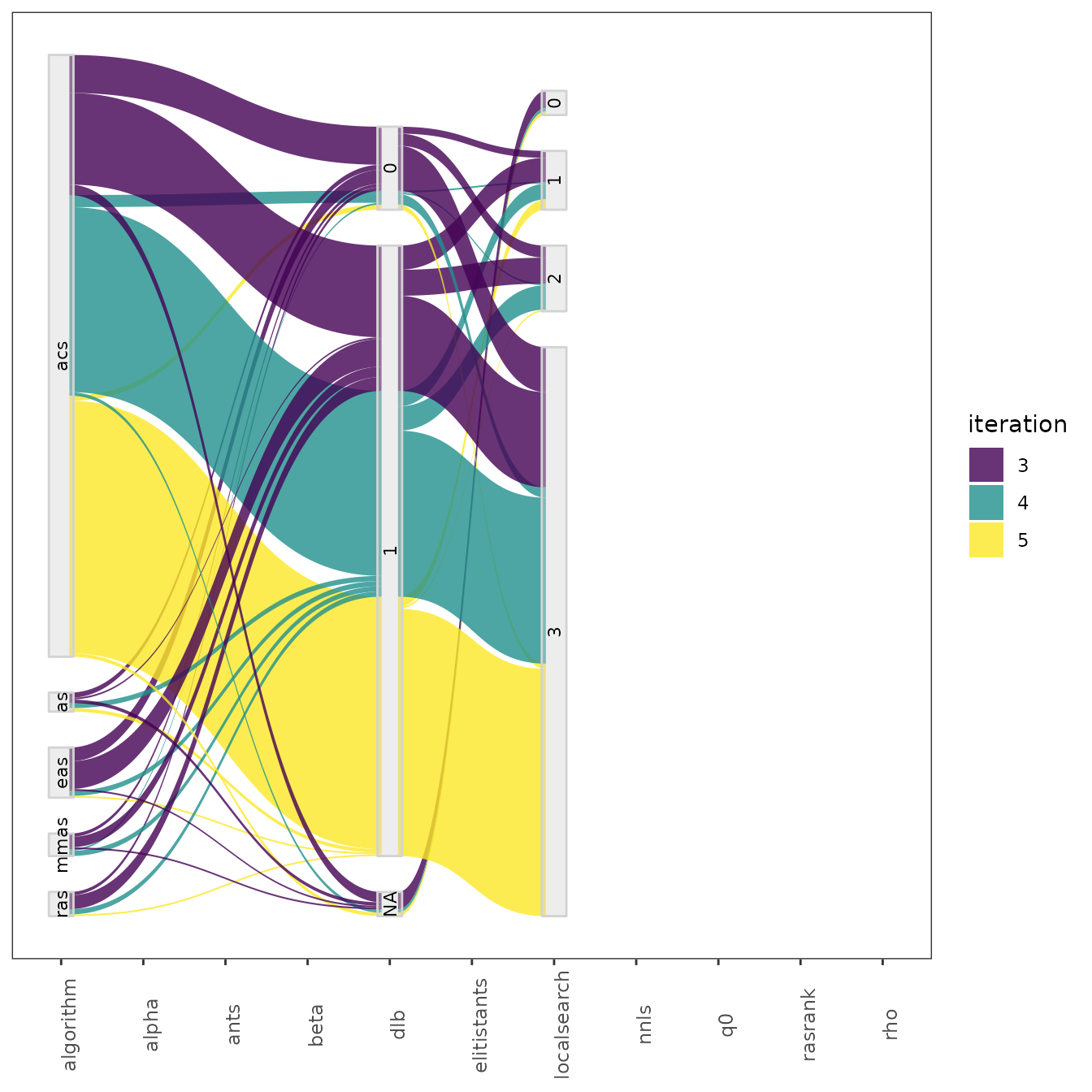
You can also adjust the number of value intervals that are displayed
for each parameter using the n_bins parameter which by
default is set to 3. Also, it is possible to select a subset of
configurations using the id_configurations argument
providing a vector a configuration ids.
Both in the parallel_coord and parallel_cat
functions parameters can be selected using the param_names
argument. For example to select parameters un
parallel_cat:
parallel_cat(irace_results = iraceResults,
             param_names=c("algorithm", "localsearch", "dlb", "nnls"))
## Warning in set(tabla, i = which(not_na), j = pname, value = bins): Coercing
## 'character' RHS to 'double' to match the type of column 5 named 'alpha'.## Warning in set(tabla, i = which(not_na), j = pname, value = bins): NAs
## introduced by coercion## Warning in set(tabla, i = which(is.na(tabla[[pname]])), j = pname, value =
## "NA"): Coercing 'character' RHS to 'double' to match the type of column 5 named
## 'alpha'.## Warning in set(tabla, i = which(is.na(tabla[[pname]])), j = pname, value =
## "NA"): NAs introduced by coercion## Warning in set(tabla, i = which(not_na), j = pname, value = bins): Coercing
## 'character' RHS to 'double' to match the type of column 6 named 'beta'.## Warning in set(tabla, i = which(not_na), j = pname, value = bins): NAs
## introduced by coercion## Warning in set(tabla, i = which(is.na(tabla[[pname]])), j = pname, value =
## "NA"): Coercing 'character' RHS to 'double' to match the type of column 6 named
## 'beta'.## Warning in set(tabla, i = which(is.na(tabla[[pname]])), j = pname, value =
## "NA"): NAs introduced by coercion## Warning in set(tabla, i = which(not_na), j = pname, value = bins): Coercing
## 'character' RHS to 'double' to match the type of column 7 named 'rho'.## Warning in set(tabla, i = which(not_na), j = pname, value = bins): NAs
## introduced by coercion## Warning in set(tabla, i = which(is.na(tabla[[pname]])), j = pname, value =
## "NA"): Coercing 'character' RHS to 'double' to match the type of column 7 named
## 'rho'.## Warning in set(tabla, i = which(is.na(tabla[[pname]])), j = pname, value =
## "NA"): NAs introduced by coercion## Warning in set(tabla, i = which(not_na), j = pname, value = bins): Coercing
## 'character' RHS to 'double' to match the type of column 8 named 'ants'.## Warning in set(tabla, i = which(not_na), j = pname, value = bins): NAs
## introduced by coercion## Warning in set(tabla, i = which(is.na(tabla[[pname]])), j = pname, value =
## "NA"): Coercing 'character' RHS to 'double' to match the type of column 8 named
## 'ants'.## Warning in set(tabla, i = which(is.na(tabla[[pname]])), j = pname, value =
## "NA"): NAs introduced by coercion## Warning in set(tabla, i = which(not_na), j = pname, value = bins): Coercing
## 'character' RHS to 'double' to match the type of column 9 named 'nnls'.## Warning in set(tabla, i = which(not_na), j = pname, value = bins): NAs
## introduced by coercion## Warning in set(tabla, i = which(is.na(tabla[[pname]])), j = pname, value =
## "NA"): Coercing 'character' RHS to 'double' to match the type of column 9 named
## 'nnls'.## Warning in set(tabla, i = which(is.na(tabla[[pname]])), j = pname, value =
## "NA"): NAs introduced by coercion## Warning in set(tabla, i = which(not_na), j = pname, value = bins): Coercing
## 'character' RHS to 'double' to match the type of column 10 named 'q0'.## Warning in set(tabla, i = which(not_na), j = pname, value = bins): NAs
## introduced by coercion## Warning in set(tabla, i = which(is.na(tabla[[pname]])), j = pname, value =
## "NA"): Coercing 'character' RHS to 'double' to match the type of column 10
## named 'q0'.## Warning in set(tabla, i = which(is.na(tabla[[pname]])), j = pname, value =
## "NA"): NAs introduced by coercion## Warning in set(tabla, i = which(not_na), j = pname, value = bins): Coercing
## 'character' RHS to 'double' to match the type of column 12 named 'rasrank'.## Warning in set(tabla, i = which(not_na), j = pname, value = bins): NAs
## introduced by coercion## Warning in set(tabla, i = which(is.na(tabla[[pname]])), j = pname, value =
## "NA"): Coercing 'character' RHS to 'double' to match the type of column 12
## named 'rasrank'.## Warning in set(tabla, i = which(is.na(tabla[[pname]])), j = pname, value =
## "NA"): NAs introduced by coercion## Warning in set(tabla, i = which(not_na), j = pname, value = bins): Coercing
## 'character' RHS to 'double' to match the type of column 13 named 'elitistants'.## Warning in set(tabla, i = which(not_na), j = pname, value = bins): NAs
## introduced by coercion## Warning in set(tabla, i = which(is.na(tabla[[pname]])), j = pname, value =
## "NA"): Coercing 'character' RHS to 'double' to match the type of column 13
## named 'elitistants'.## Warning in set(tabla, i = which(is.na(tabla[[pname]])), j = pname, value =
## "NA"): NAs introduced by coercion## Warning: Removed 124 rows containing non-finite outside the scale range
## (`stat_parallel_sets()`).## Warning: Removed 124 rows containing non-finite outside the scale range
## (`stat_parallel_sets_axes()`).
## Removed 124 rows containing non-finite outside the scale range
## (`stat_parallel_sets_axes()`).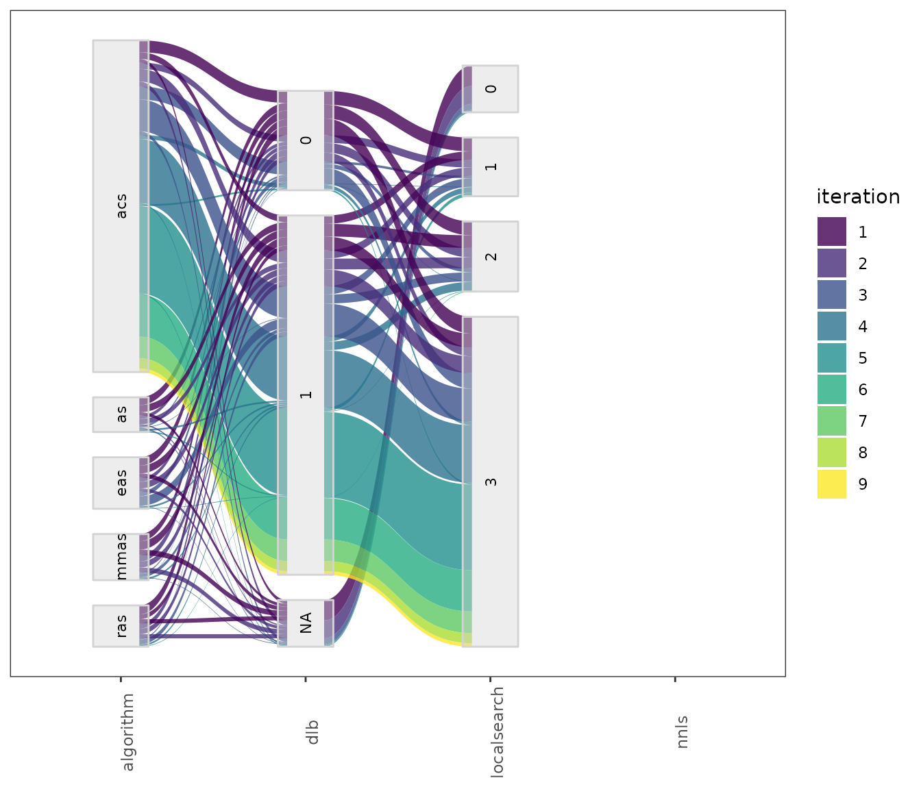
This setting is useful to visualize the association between
parameters that, for example, seem to interact. For configuration
scenarios that define a large number of parameters, it is impossible to
visualize all parameters in one of these plots. If do not know which
parameters to select, all parameters can be split in different plots
using the by_n_param argument which specifies the maximum
number of parameters to include in a plot. The functions will generate
as many plots as needed to cover all parameters included.
Sampled values and frecuencies
The sampling_pie function creates a plot that displays
the values of all configurations sampled during the configuration
process. This plot can be useful to display the tendencies in the
sampling in a simple format. As well as in the
previousparallel_cat` plot, numerical parameters domains
are discretized to be shown in the plot. The size of each parameter
value in the plot is dependent of the number of configurations having
that value in the configurations.
sampling_pie(irace_results = iraceResults)As in previous plots, you can select the parameters to display with
the param_names argument and the number of intervals of
each parameter with the n_bins argument. The generated plot
is interactive, you can click in each parameter to display it
independently.
In some cases in might be interesting to have a look at the values
sampled during the configuration procedure as a distribution. Such plot
shows the areas in the parameter space where irace detected a high
performance. A general overview of the distribution of sampled
parameters values can be obtained with the
sampling_frequencyfunction which generates frequency and
density plots for the sampled values:
sampling_frequency(iraceResults)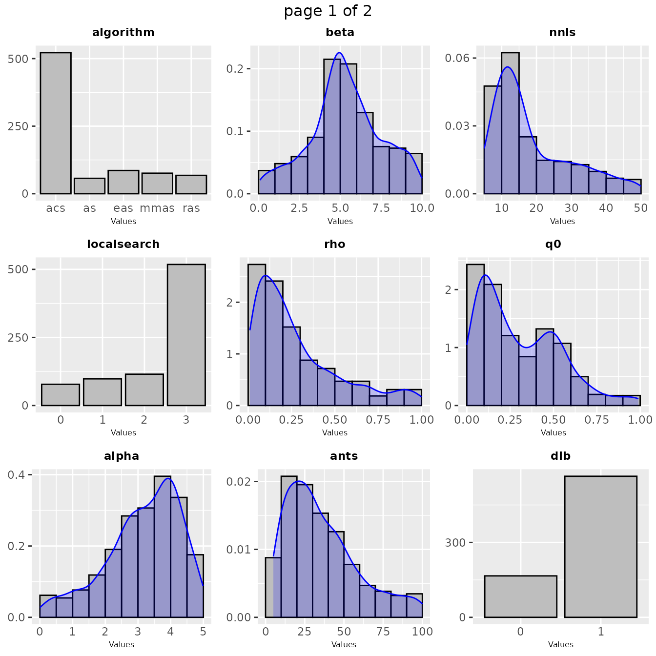
If you would like to visualize the distribution of a particular set
of configurations, you can pass directly a set of configurations and a
parameters object in the irace format to the
sampling_frequency function:
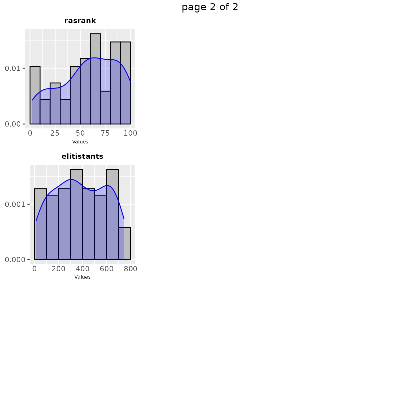
sampling_frequency(iraceResults$allConfigurations, iraceResults$scenario$parameters)The previous functions display the parameter frequency plots grouped
by 9 plots, you can adjust this setting using the n
argument. You can select the parameters to be displayed, with the
param_names argument. You can use these plots to ge a
general idea of the area of the parameter space in which the sampling
performed by irace was focused. For example:
sampling_frequency(iraceResults, param_names = c("beta"))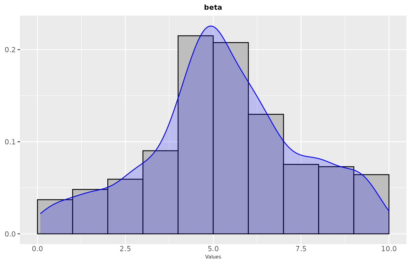
If you would like to see more details, a plot showing the sampling by
iteration can be obtained with the
sampling_frequency_iterationfunction. This plot shows the
convergence of the configuration process reflected in the parameter
values sampled each iteration:
sampling_frequency_iteration(iraceResults, param_name = "beta")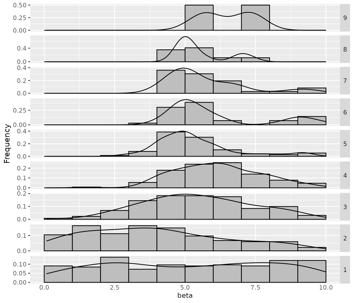
In some cases, you may want to assess how the sampling frequencies of
two parameters are related. You can visualize the joint sampling
frequency of two parameters using the sampling_heatmap
function. By default, this plot uses the elite configurations values (of
all configurations), you can allow the plot to show all sampled
configurations using the only_elite argument. You must
select two parameters using the param_names argument, for
example:
sampling_heatmap(iraceResults, param_names = c("beta","alpha"))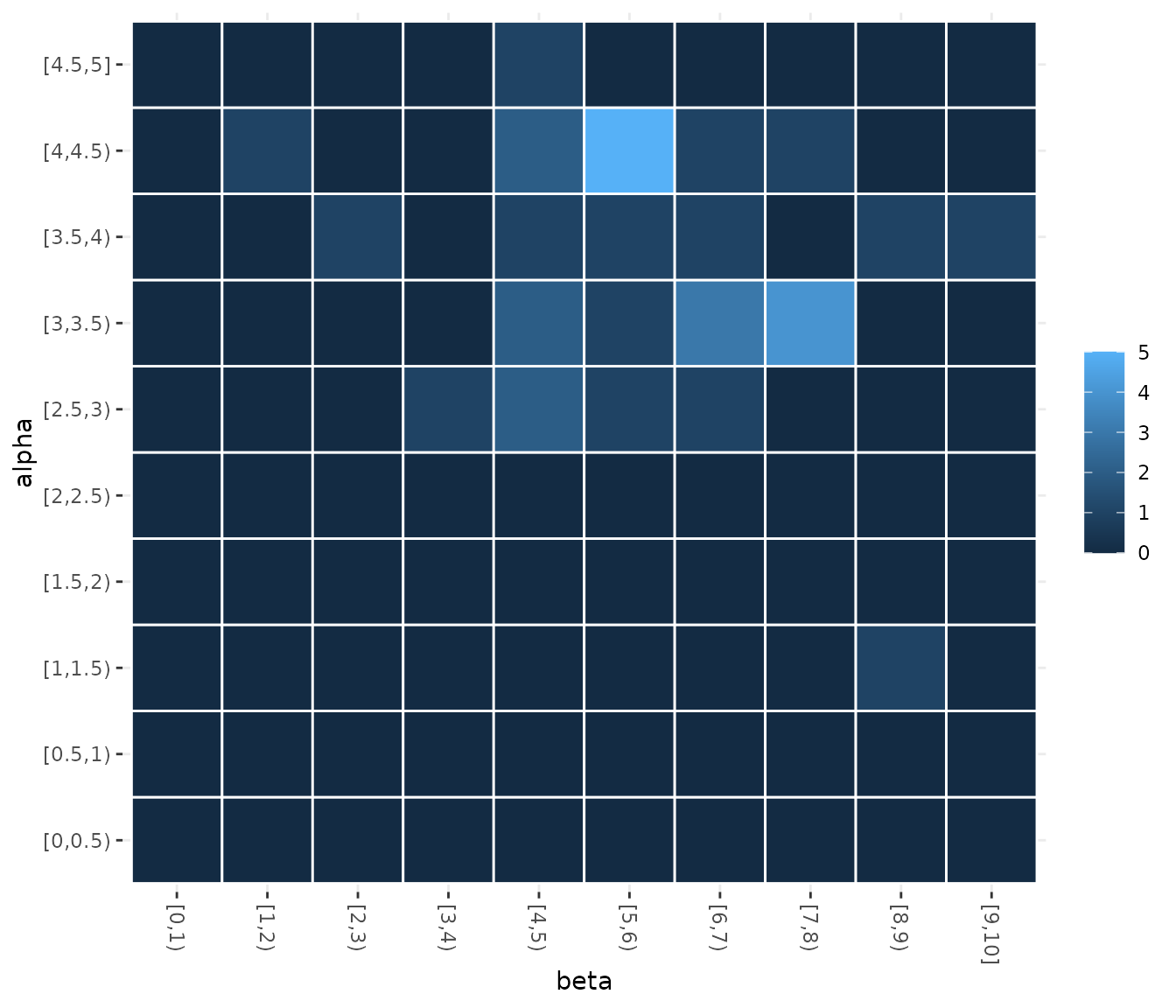
You can also select the iterations from which configurations will be
selected using the iterations argument. The size of the
intervals considered for numerical parameters in the heatmap can be also
adjusted, see the example to have more details.
If you would like to display a set of configurations directly
provided by you, use the sampling_heatmap2 function. In
both sampling_heatmap2 and sampling_heatmap2,
you can adjust the number of intervals to be displayed for numerical
parameters using the sizes argument. For example, we set to
5 the number of intervals displayed for the second parameter, which is
numerical, using sizes=c(0,5). The the 0 value in this
argument indicates that the default interval size should be used. In
this case, we set 0 for the first parameter but note that it is not
possible to adjust the number of intervals for categorical or ordered
parameter types.
sampling_heatmap2(iraceResults$allConfigurations, iraceResults$scenario$parameters,
                  param_names = c("localsearch","nnls"), sizes=c(0,5))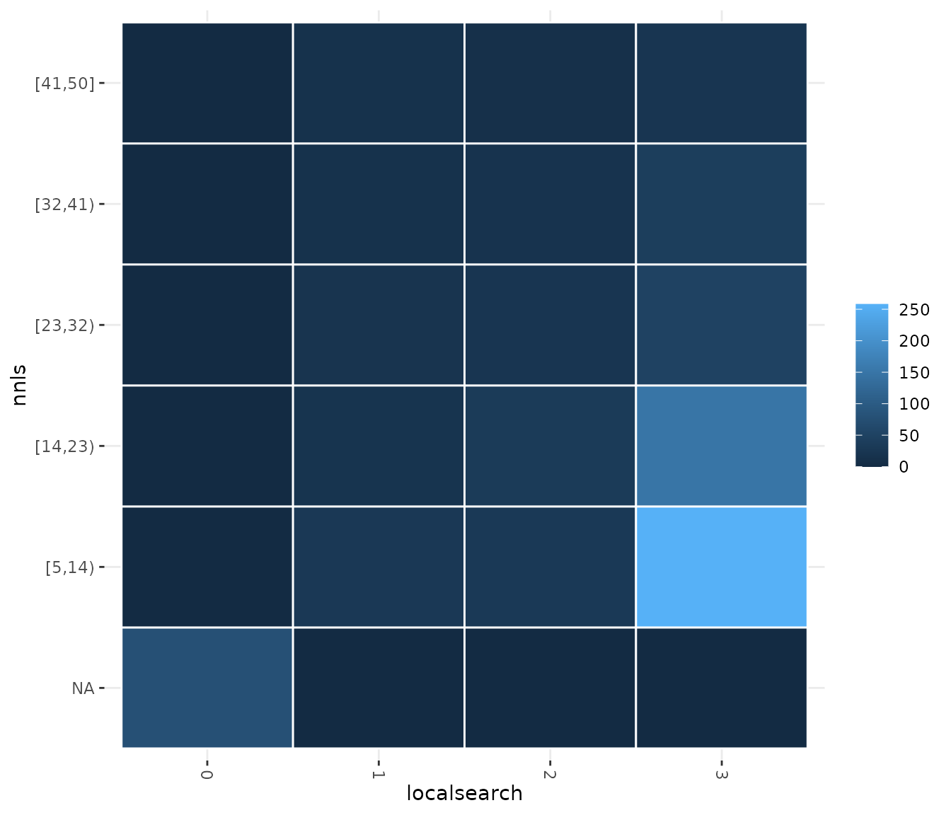
Sampling distance
You may like to have a general overview of the distance of the
configurations sampled across the configuration process. This can allow
you to assess the convergence of the configuration process. The mean
distance between the sampled configurations can be visualized using the
sampling_distance function. This function compares the
parameter values of all configurations and aggregates these comparisons
to calculate the overall distance:
sampling_distance(iraceResults, t=0.05)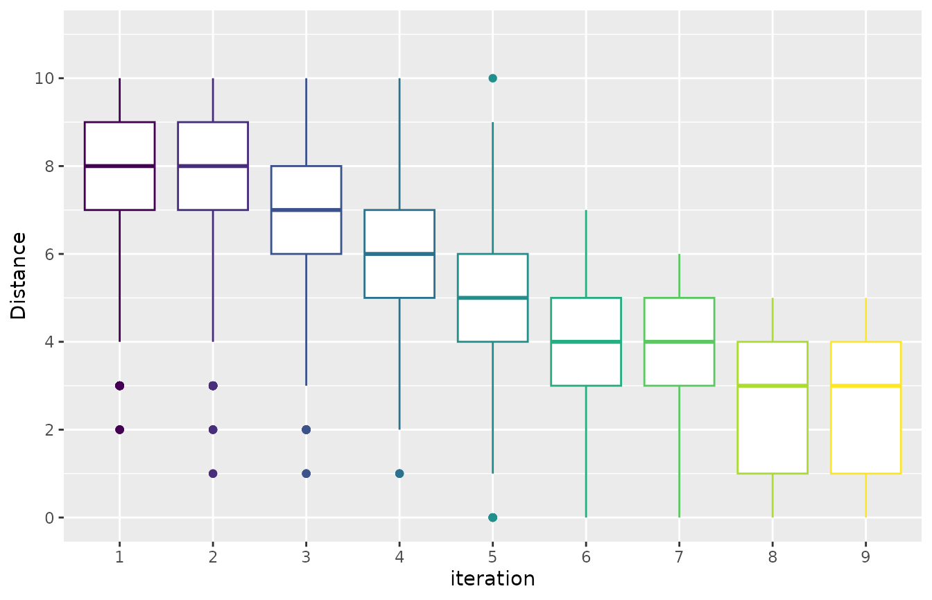
Note that for categorical and ordered parameters the comparison is
straightforward, but this is not the case for numerical parameters. The
argument t defines a percentage used to define a domain
interval to assess equality of numerical parameters. For example, if the
domain of a parameter is [0,10] and t=0.1 then
when comparing any value to v=2 we define an interval
s=t* (upper_bound -lower_bound) = 0.1*(10-0)=1. Then all
values in the interval [v-s, v+s] [1,3] will be equal to
v=2.
Visualizing Performance
Test performance (elite configurations)
When executing irace, you can enable the testing feature that will evaluate elite configurations in a set of test instances. For more details about how you can use this feature check the irace package user guide.
The test performance of the evaluated configurations can be
visualised using the boxplot_test function. Note that the
irace execution log file includes test data (test is not enabled by
default).
boxplot_test(iraceResults, type="best")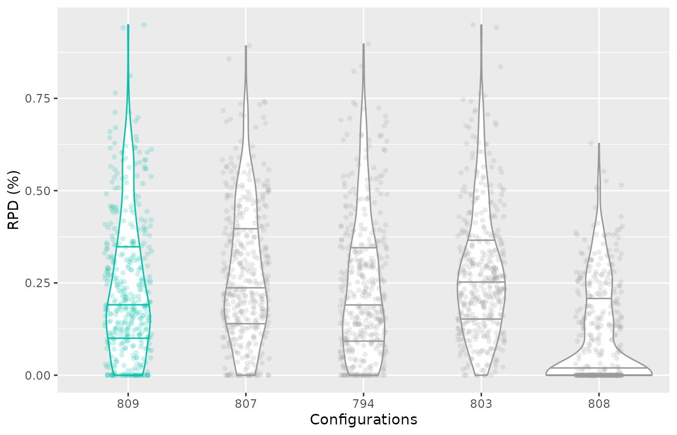
This plot shows all final elite configurations evaluation on the test
instance set, we can compare the performance of these configurations to
select one that has the best test performance. Note that the best
configuration (identified by irace) is displayed in a different color.
By default, the plot displayes the relative percentage deviation of the
performance of the configurations, to disable this and display the raw
performance use the rpd=FALSE argument.
If the irace log file includes the evaluation on the test set of the
iteration elite configurations, its possible to plot the test
performance of elite configurations across the iterations using the
argument type="all". The best elite configuration on each
iteration is displayed in different color:
boxplot_test(iraceResults, type="all", show_points=FALSE)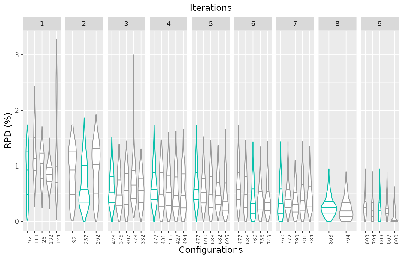
This plot allows to assess the progress of the configuration process regarding the test set performance, which would be useful when dealing with heterogeneous instance sets. In these cases, good configurations across the full set can be challenging to find and it is possible that the algorithm could be mislead if instances sets are prone to introduce bias due to instance ordering.
Note that in this example the elite configuration with id 808 seems
to have a slightly better performance
than the configuration identified as the best (id:809) by irace. It is
important to note that all elite configurations are not statistically
different and thus, its very possible that such situation is observed
when evaluuting test performance, specially when configuring
heterogeneous, difficult to balance, instance sets.
If you would like further detauls about the difference in the
performance of two configurations, you can use the
scatter_test function. This function displays the
performance of both configurations paired by instance (each point
represents an instance):
scatter_test(iraceResults, x_id = 808, y_id = 809, interactive=TRUE, instance_names = basename)If the plot is created using the argument
interactive=TRUE you can visualize the instance name when
placing the cursor over each performance point. This plot can help to
identify subsets of instances in which a configuration clearly
outperforms other. To further understand the difference of these two
configurations the trainig data might be explored to verify if such
effect holds for the training set.
Training performance (all configurations)
During the execution of irace considerable performance data is obtained in order to assess the performance of the candidate configurations. This data can be useful to understand the performance of the configured algorithm and to get insights about how to improve the configuration process.
The following functions create plots of the training data in the irace log. Note that this data is obtained during the search of good configurations. Due to the racing procedure, some configurations are more evaluated than others (best configurations are more evaluated than poor performing configurations). See the irace package documentation for details.
Visualizing training performance might help to obtain insights about the reasoning that followed irace when searching the parameter space, and thus it can be used to understand why irace considers certain configurations as high or low performing.
To visualize the performance of the final elites as observed by
irace, the boxplot_training function plots the experiments
performed on these configurations. Note that this data corresponds to
the performance generated during the configuration process thus, the
number of instances on which the configurations were evaluated might
vary between elite configurations.
boxplot_training(iraceResults)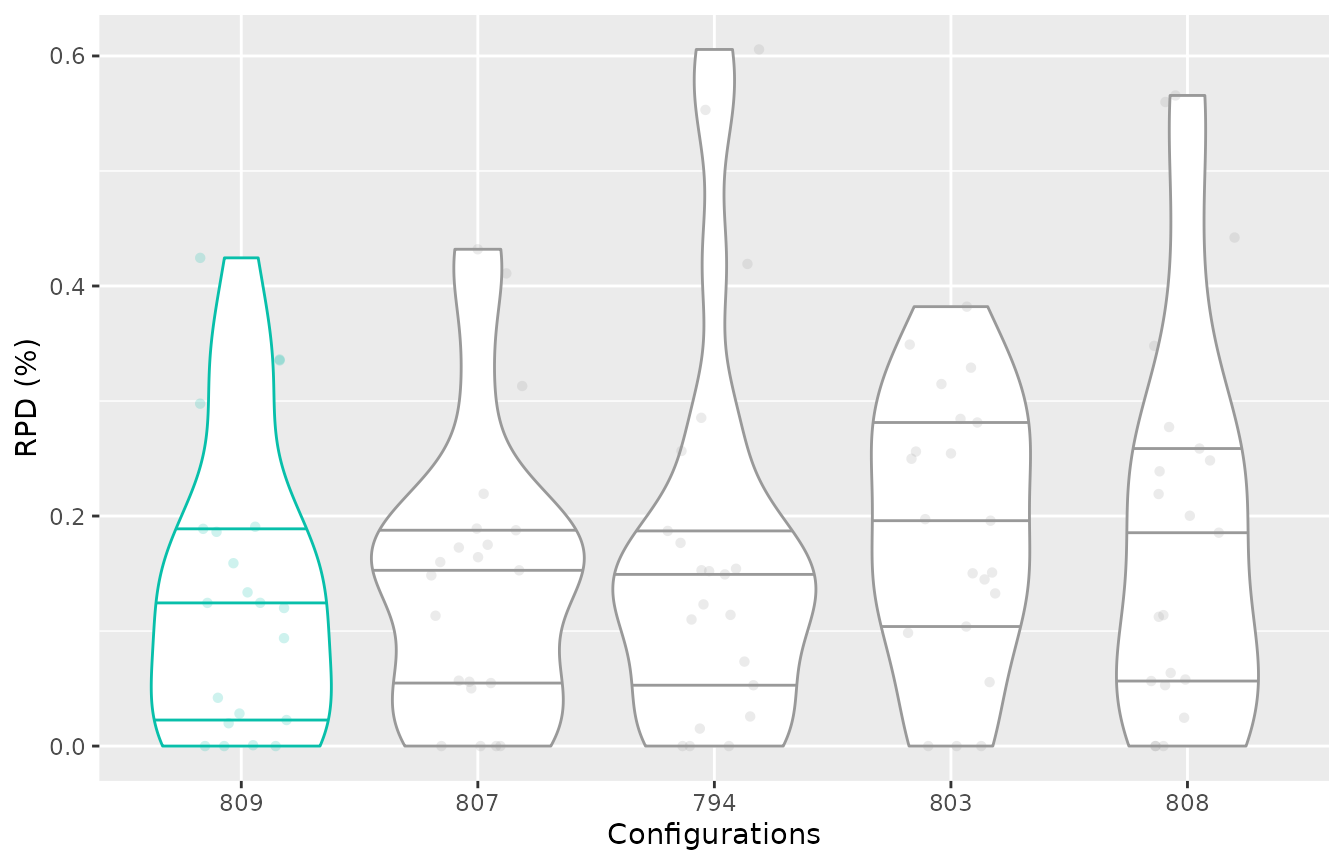
You can select to display the elite configurations of a different
iteration by using the iteration. In case you would like to
visualize non-elite configurations you can directly provide the instance
ids using the `. This can be very useful to assess the performance of
initial configurations provided for the configuration process for
example, providing insights about why irace did not select them as final
elite configurations:
iteration_elites = iraceResults$iterationElites
boxplot_training(iraceResults, id_configurations=c(1, iteration_elites))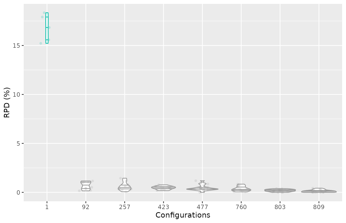
To visualize the difference in the performance of two configurations
you can also generate a scatter plot using the
scatter_training function:
scatter_training(iraceResults, x_id = 808, y_id = 809, interactive=TRUE)If the plot is created using the argument
interactive=TRUE you can visualize the instance name when
placing the cursor over each performance point.
For both functions boxplot_training and
scatter_training, you can display either the relative
percentage deviation (rpd=TRUE) or the raw performance
(rpd=FALSE).
You can also plot the performance of configurations which was not necessarily obtained when executing irace. Check the General purpose performance section for details.
General purpose performance
You can use the following functions to plot the performance of a selected set of configurations in an experiment matrix provided directly by you. These functions can be also useful when you would like to compare a configuration that was not generated in the configuration process. Note thar such comparison should be carefully considered as execution conditions might differ from the ones when irace was executed. Keep in mind that irace provides seeds to execute instances when configuring stochastic algorithms and also might define an execution bound when adaptive capping is active. Check the irace package user guide for details about this.
To plot the performance of a selected set of configurations in an
experiment matrix, you can use the boxplot_performance
function. The configurations can be selected in a vector
(allElites):
boxplot_performance(iraceResults$experiments, allElites=c(800, 803,808,809))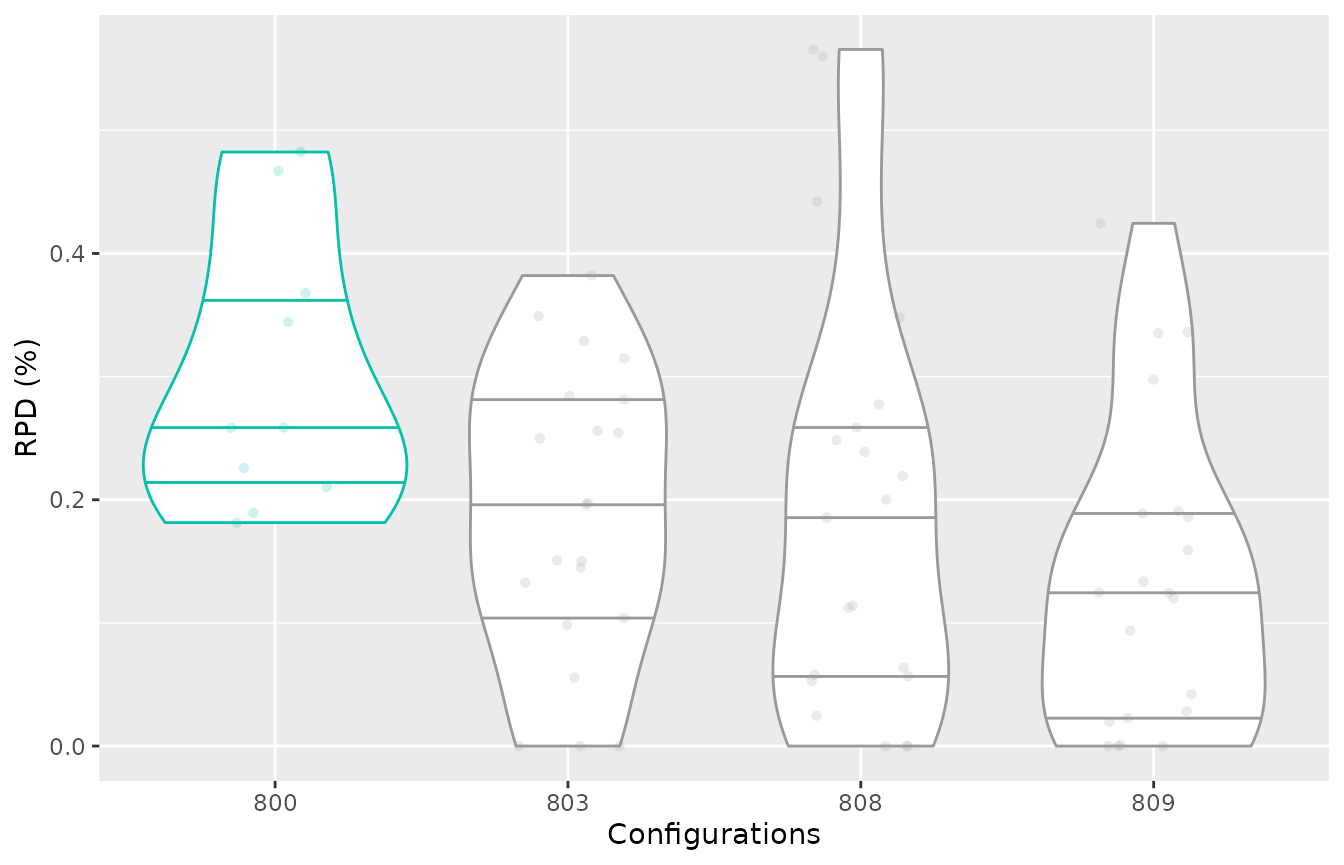
The experiment matrix should be provided in the irace format, columns should have configuration ids as names (character) and rows names can be instances names (optional).
If the configurations are provided in a list, then the different
elements of this list will be considered as iterations. Note that this
matches the iraceResults$allElites variable in the irace
log. For example, to plot 3 configurations as they are assigned to 3
different iterations:
boxplot_performance(iraceResults$experiments, allElites=as.list(c(800,803,808,809)))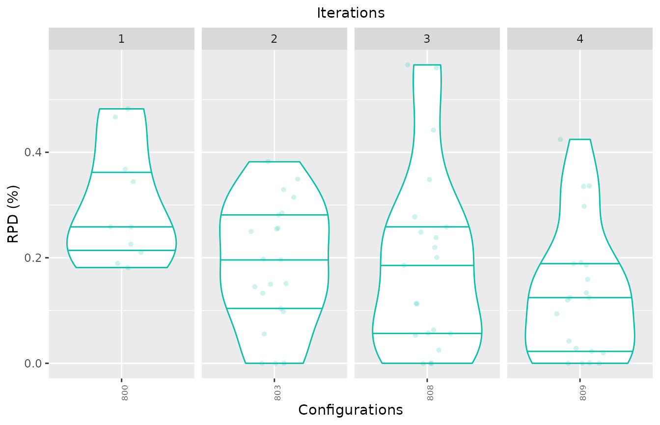
Each element of a list can have more than one id (vector). You can
place at the start of each vector the configuration id you want to be
identified as the best one and use first_is_best = TRUE to
have it displayed in the different color. Adjust the color using the
best_color argument.
boxplot_performance(iraceResults$experiments, allElites=list(c(803,808), c(809,800)), first_is_best = TRUE)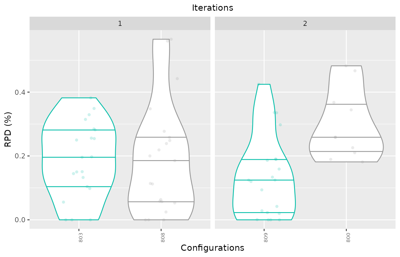
If you want to further compare the performance of two configurtions,
you can use the scatter_perfomance function to plot the
difference between configurations:
scatter_performance(iraceResults$experiments, x_id = 803, y_id = 809, interactive=TRUE, instance_names = basename)If the plot is created using the argument
interactive=TRUE and, the provided matrix has row names,
you can visualize the instance name when placing the cursor over each
performance point otherwise an instance ID is displayed. In this
example, we further transform instance names using the function
basename().
Visualizing the configuration process
In some cases, it might be interesting have a general visualization
for the configuration process progress. This can be generated with the
plot_experiments_matrix function:
plot_experiments_matrix(iraceResults, interactive = TRUE)This plot shows configurations in the x axis and instances in the y
axis. Each point in the plot display in color the ranking of the
configuration on each instance. If interactive = TRUE, you
can place your cursor on each point to visualize the configuration id,
instance id, and the rank of the configuration.
The sampling distributions used by irace during the configuration
process can be displayed using the plot_model function. For
categorical parameters, this function displays the sampling
probabilities associated to each parameter value by iteration (x axis
top) in each elite configuration model (bars):
plot_model(iraceResults, param_name="algorithm")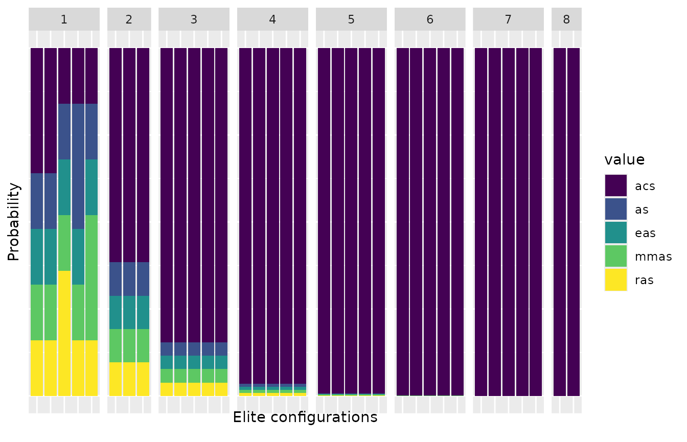
For numerical parameters, this function shows the sampling distributions associated to each parameter. These plots display the the density function of the truncated normal distribution associated to the models of each elite configuration in each instance:
plot_model(iraceResults, param_name="alpha")## Warning: Using `size` aesthetic for lines was deprecated in ggplot2 3.4.0.
## ℹ Please use `linewidth` instead.
## ℹ The deprecated feature was likely used in the iraceplot package.
## Please report the issue at
## <https://github.com/auto-optimization/iraceplot/issues>.
## This warning is displayed once every 8 hours.
## Call `lifecycle::last_lifecycle_warnings()` to see where this warning was
## generated.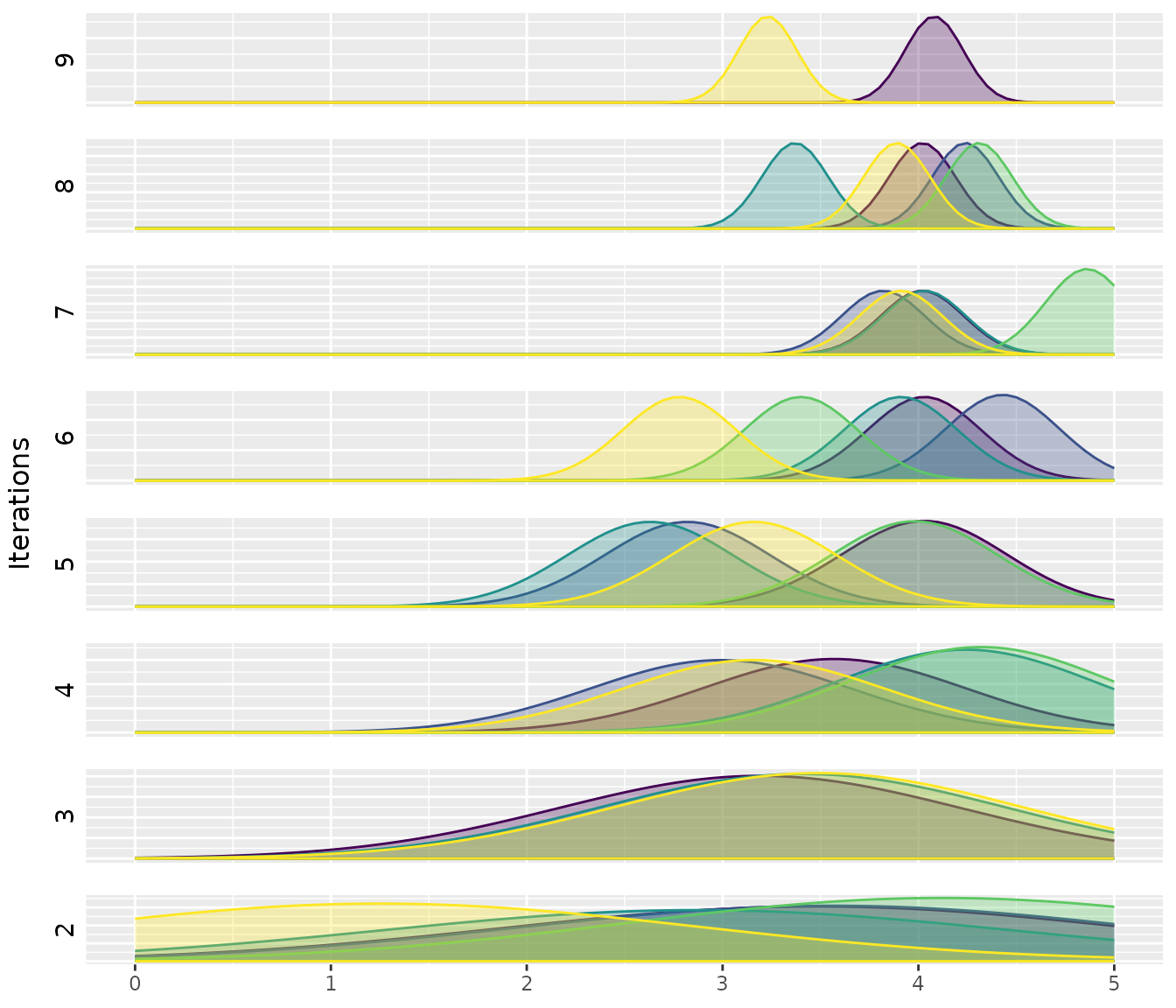
Report
If you want a quick and portable overview of the configuration
process, you can use the report function which generates an
HTML report with a summary of the configuration process executed by
irace. The function will create an HTML file in the path provided in the
filename argument and appending the ".html"
extension to it.
report(iraceResults, filename="report")